How to Freeze Multiple Rows and or Columns in Excel using Freeze Panes. Right click on it and hide itStep 2.
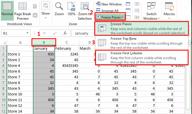
2 Examples Of How To Freeze First And Multiple Columns In Excel
We can freeze the middle row of the excel worksheet as your top row.
Freeze top three rows in excel. Jan 25 2021 Select the rows and click on view from the menu bar. Microsoft excel has three options to help you freeze the rows and columns via the freeze panes menu. Introduction to Functions and Formulas.
To lock columns select the column to the right of where you want the split to appear To lock both rows and columns click the cell below and to the right of where you want the split to appear. Go to the View tab followed by clicking on the Freeze Panes option. Freeze rows or columns Select the third column.
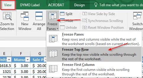
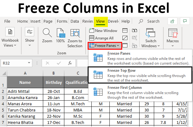
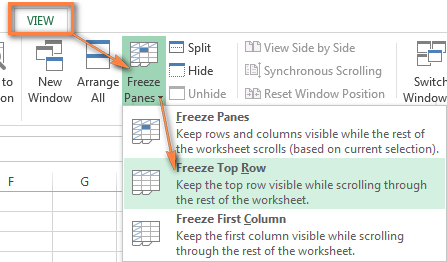
Freeze Top Row Freezes only the top row of our Excel file. Are you saying if you do that it only does the top 2 rows. Replied on February 15 2013.
To lock the top-most row only select cell A2 the entire row 2 or use the Freeze Top Row option available in the Freeze Panes drop-down menu on the View tab 22. For example if you wish to lock the top two rows place the mouse cursor in cell A3 or select the entire row 3. If you place a cursor in the unknown cell and freeze multiple rows then you may go wrong in freezing.
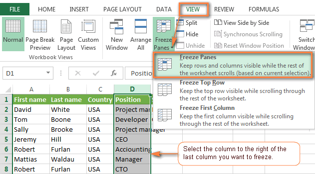
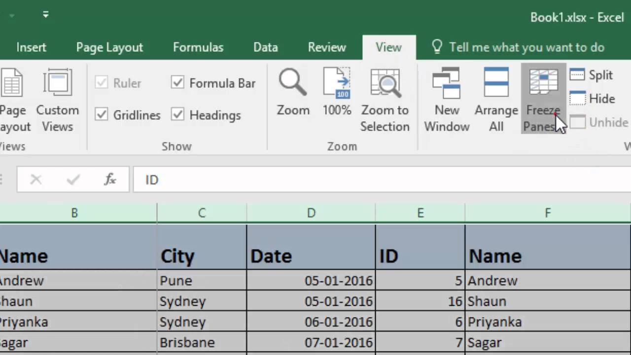
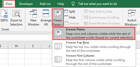
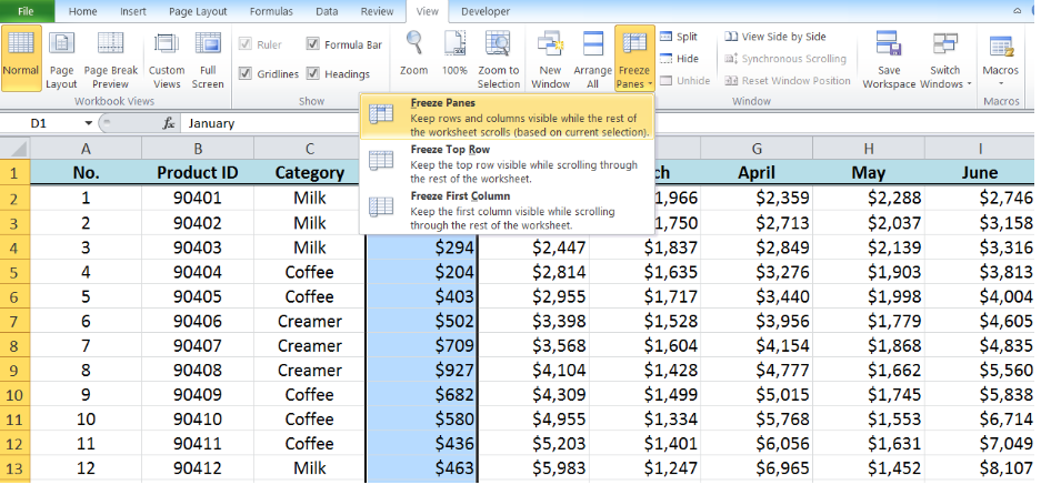
To freeze multiple columns select the column to the right of the last column you want frozen and click Freeze Panes. You have frozen the multiple rows in excel 2019. Freeze Panes Keeps rows and columns visible while the rest of the worksheet scrolls based on current selection.
Open an excel file and go to the view tab. Last two option seems logical. Under Menu go to View Free.
Instructions on how to freeze the top 3 rows on ExcelStep 1. Freeze the top row. The result will be similar to what you see in the screenshot below - the top 2 rows in your Excel worksheet are frozen and will always show up.
Youd select cell D5 and then on the View tab click Freeze Panes. Freeze or unfreeze rows. Open the Worksheet you want to work on.
A list of options appears to select the option of freeze panes which is the first option. Under view search for freeze panes. Freeze rows or columns Select the cell below the rows and to the right of the columns you want to keep visible when you scroll.
It should be click in cell A4 and then View - Freeze Panes. This will lock the very first row in your worksheet so that it remains visible when you navigate through the rest of your worksheet. This guide will show you a step-by-step approach in freezing the top 3 rows in Excel.
Select View Freeze Panes Hide or show rows or columns Freeze panes to lock the first 1. How to freeze 3 Rows in Excel Basic Excel Tutorial. Under view search for freeze panes and click on it.
Quickly combine merge multiple columns or rows in Excel. Select the row or the first cell in the row located right below the row that contains the column headings. Make sure you have selected the right cell to freeze.
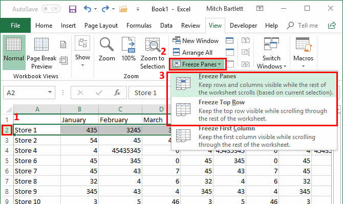
Make sure the filter is removed while freezing multiple rows at a time. With the row selected click on the View tab at the top select Freeze Panes and youll see several different options you can choose. Freeze pane the top row.
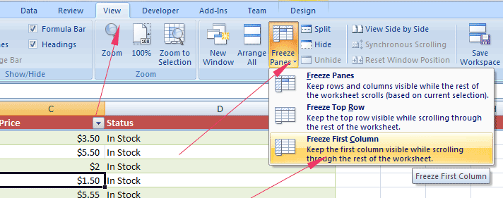
Freeze First Column Freezez only the first column in our Excel file. Select the cell below the rows and to the right of the columns you want to keep visible when you scroll. Open the sheet where in you want to freeze any row header as an example we would like to freeze the top row highlighted in yellow.
Select View Freeze Panes Freeze Panes. The Dropdown menu of Freeze Panes has three options. After that click on the view tab now click on freeze panes and then again freeze panes.
Head over to the View tab and click Freeze Panes Freeze Panes. 32 people found this reply helpful. To lock top row in Excel go to the View tab Window group and click Freeze Panes Freeze Top Row.
Select the View tab and navigate to Freeze Panes. Select View Freeze Panes Freeze Panes. Here is a tutorial on how to freeze three rows on your excel worksheet.
Click on freeze panes a list of three options will 21. Select Freeze Top Row option. On the View tab in the Window group click Freeze Panes.
First select the below cell of the rows that you want to freeze like if you want to freeze the first two rows then select the cell of the third row from the first column. Say you want to freeze the top four rows and leftmost three columns. For example you select the cell C3.
Click on the Freeze Panes button. Click on the Freeze Panes option which is situated at the top in the drop-down menu. The freeze a pane option on excel will assist you in this task.
Highlight the first two rows. How to freeze top row in Excel. Freezing of three rows on Excel spreadsheet.
We are going to highlight the first four rows because they are the ones we wish to lock after that we go to the menu bar and click on view. Now navigate to the View tab in the Excel Ribbon as shown in above image.
How To Freeze Panes In Excel Lock Rows And Columns Ablebits Com
Microsoft Excel Freeze Or Unfreeze Panes Columns And Rows
How To Freeze Multiple Columns In Microsoft Excel Youtube

Excel Freeze Panes To Lock Rows And Columns

Freeze And Split Panes In Ms Excel Tech Savvy
Freeze Columns In Excel Examples On How To Freeze Columns In Excel
Freeze Multiple Rows When Scrolling Excel For Mac Lasoparuby
How To Lock Or Freeze Row Or Column In Excel Free Excel Tutorial
How To Freeze Rows And Columns In Google Sheets And Excel Excelchat
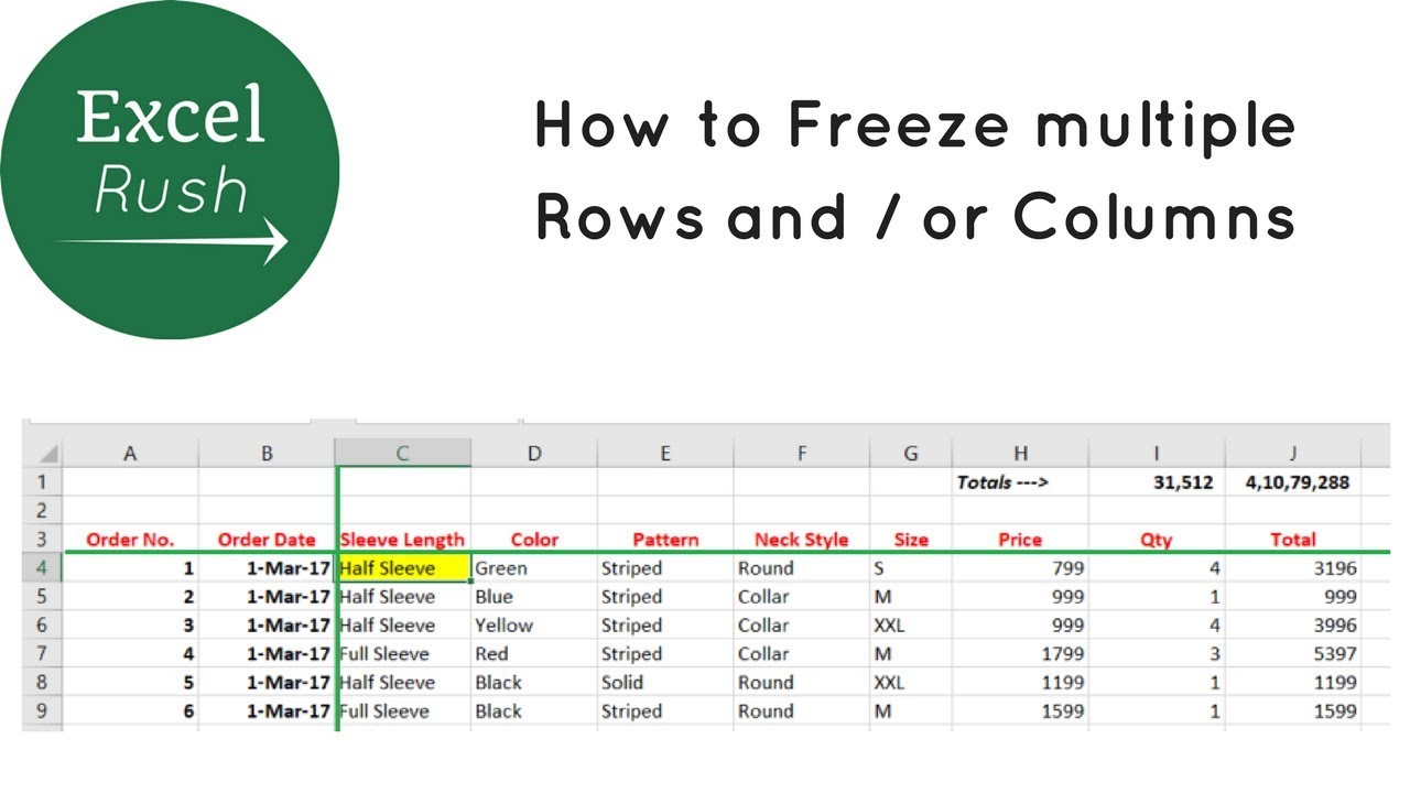
How To Freeze Multiple Rows And Or Columns In Excel Using Freeze Panes Youtube
Microsoft Excel Freeze Or Unfreeze Panes Columns And Rows

How To Freeze Header Rows Or Columns In Excel

How To Freeze 3 Rows In Excel Basic Excel Tutorial
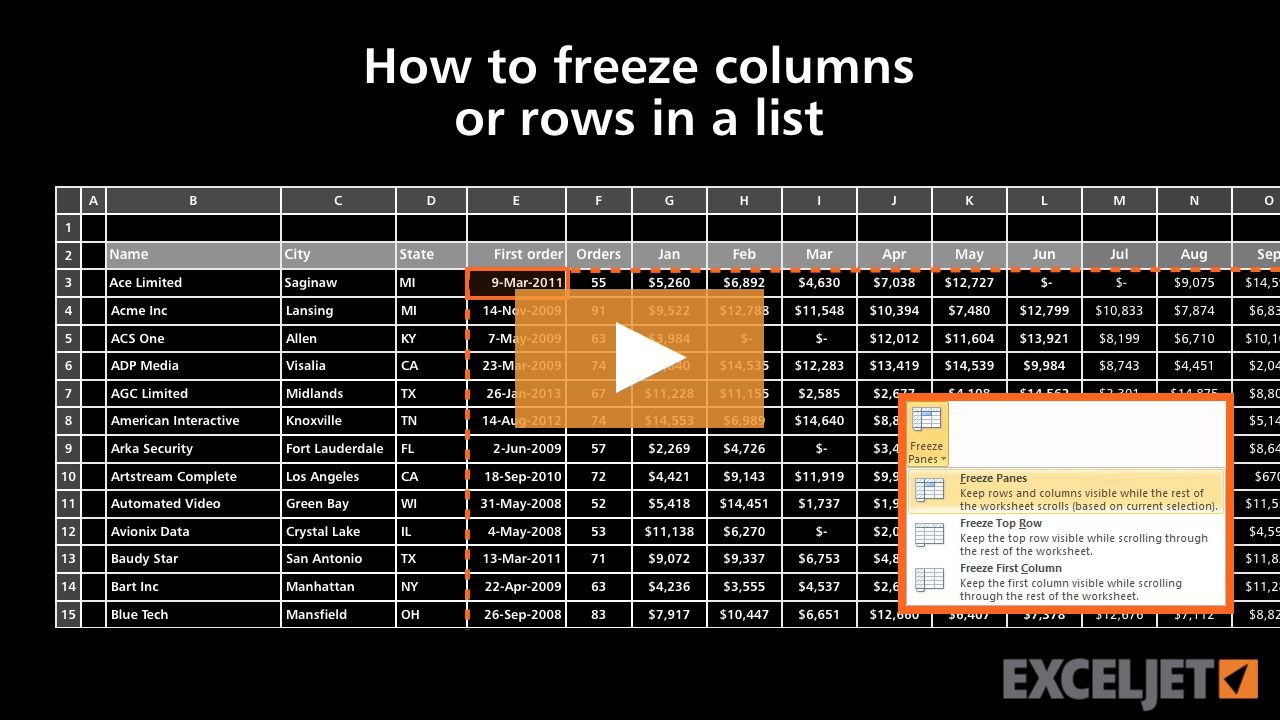
Excel Tutorial How To Freeze Columns Or Rows In A List

How To Freeze 3 Rows In Excel Basic Excel Tutorial

Excel 2010 Freeze Rows And Columns
How To Freeze Panes In Excel Lock Rows And Columns Ablebits Com

How To Freeze Rows And Columns In Excel Guide By Learn Army
Tech Tip Freezing Rows And Columns In Excel Weston Technology Solutions
